How to Calculate Volatility A Trader's Guide
Calculating volatility is all about measuring how much an asset's price jumps around. The go-to method is finding the standard deviation of its price changes over a set period. This number gives you a direct, quantifiable measure of risk and the potential for big swings.
We'll break down how to calculate both historical volatility (what happened in the past) and implied volatility (what the market expects to happen next).
Why Volatility Is a Trader's Most Important Metric
Before we jump into the math, let's get one thing straight: volatility isn't just a fancy word for "choppy markets." It's the language of risk and opportunity. If you don't speak it, you're just guessing.
Getting a real handle on volatility is what separates data-driven decisions from gut feelings.
Think of it this way. You can drive from point A to point B on a straight, clear highway or a winding mountain road in a blizzard. One requires a lot more skill and attention to risk. Trading without understanding volatility is like heading into that blizzard without checking the weather forecast—you might be fine, but you could also drive straight into disaster.
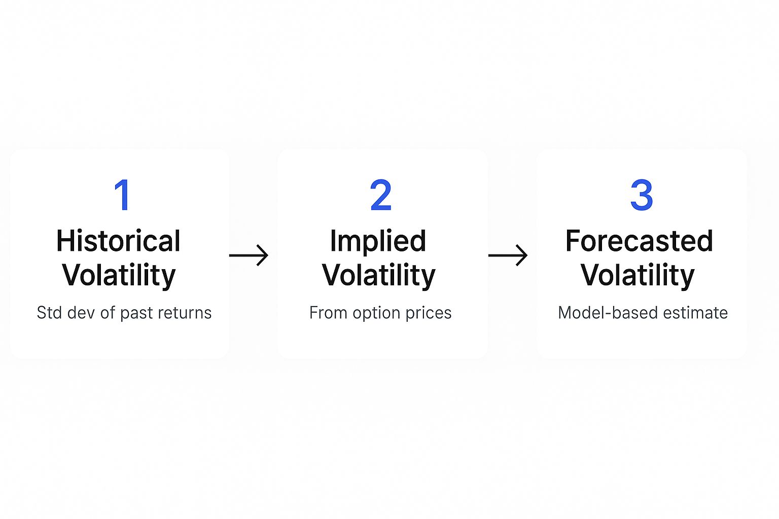
The Two Faces of Volatility
To really get it, you need to know its two main forms. Each one tells you a different part of the story, and smart traders use both to build a complete picture of what the market is doing.
- Historical Volatility (HV): This is purely backward-looking. It tells you how much an asset’s price has moved in the past. It's calculated from old price data and gives you a baseline for what's "normal" for that asset.
- Implied Volatility (IV): This is forward-looking and is pulled from options prices. IV represents the market's collective bet on how volatile an asset will be in the future. The famous VIX index, or "fear gauge," is just a measure of implied volatility for the S&P 500.
To give you a clearer sense of how these two metrics differ and what they're used for, here’s a quick side-by-side comparison.
Historical vs Implied Volatility At a Glance
| Attribute | Historical Volatility | Implied Volatility |
|---|---|---|
| Perspective | Backward-looking | Forward-looking |
| Data Source | Past price data of the asset | Current options prices |
| What It Measures | Actual, realized price movement | Market's expectation of future movement |
| Primary Use | Assessing past risk, setting baselines | Pricing options, gauging market sentiment |
| Common Analogy | Looking in the rearview mirror | Looking at the road ahead |
Understanding the interplay between past performance and future expectations is where the real edge lies. One tells you where you've been, the other where the market thinks you're going.
Here's something I've learned over the years: volatility clusters. Wild periods are often followed by more wildness, and calm periods tend to stick around for a while. Being able to spot which "regime" you're in is critical for adapting your strategy on the fly.
From Theory to Practical Application
Knowing an asset's volatility helps you do practical things, like setting smarter stop-losses, figuring out the right position size, and spotting potential breakout trades. An asset with volatility spiking higher might be winding up for a big move. If it's shrinking, it could be settling into a quiet consolidation phase.
This concept is also fundamental when you're learning how to diversify a portfolio effectively, as it helps you balance high-risk and low-risk assets.
By mastering the calculations we're about to cover, you're not just learning a formula. You're building a core skill for navigating the markets with more confidence and control. It’s the bedrock of solid risk management and sharp trade planning.
Your First Volatility Calculation with Closing Prices
Alright, let's jump in and calculate historical volatility the classic way. This is the most direct method for seeing how much an asset’s price has bounced around in the past, and it gives you a solid baseline for understanding its risk. The best part? You can use this approach for pretty much anything, from a tech giant like Tesla (TSLA) to Bitcoin (BTC).
The core idea is simple. We're going to measure the standard deviation of the asset's daily returns. Specifically, we'll use the common 'Close-to-Close' method, which just means we're looking at the percentage change from one day's closing price to the next.
Once we have that daily volatility figure, we'll annualize it by multiplying it by the square root of the number of trading days in a year—which is typically 252. You can learn more about estimating past volatility with this method if you want to go deeper.
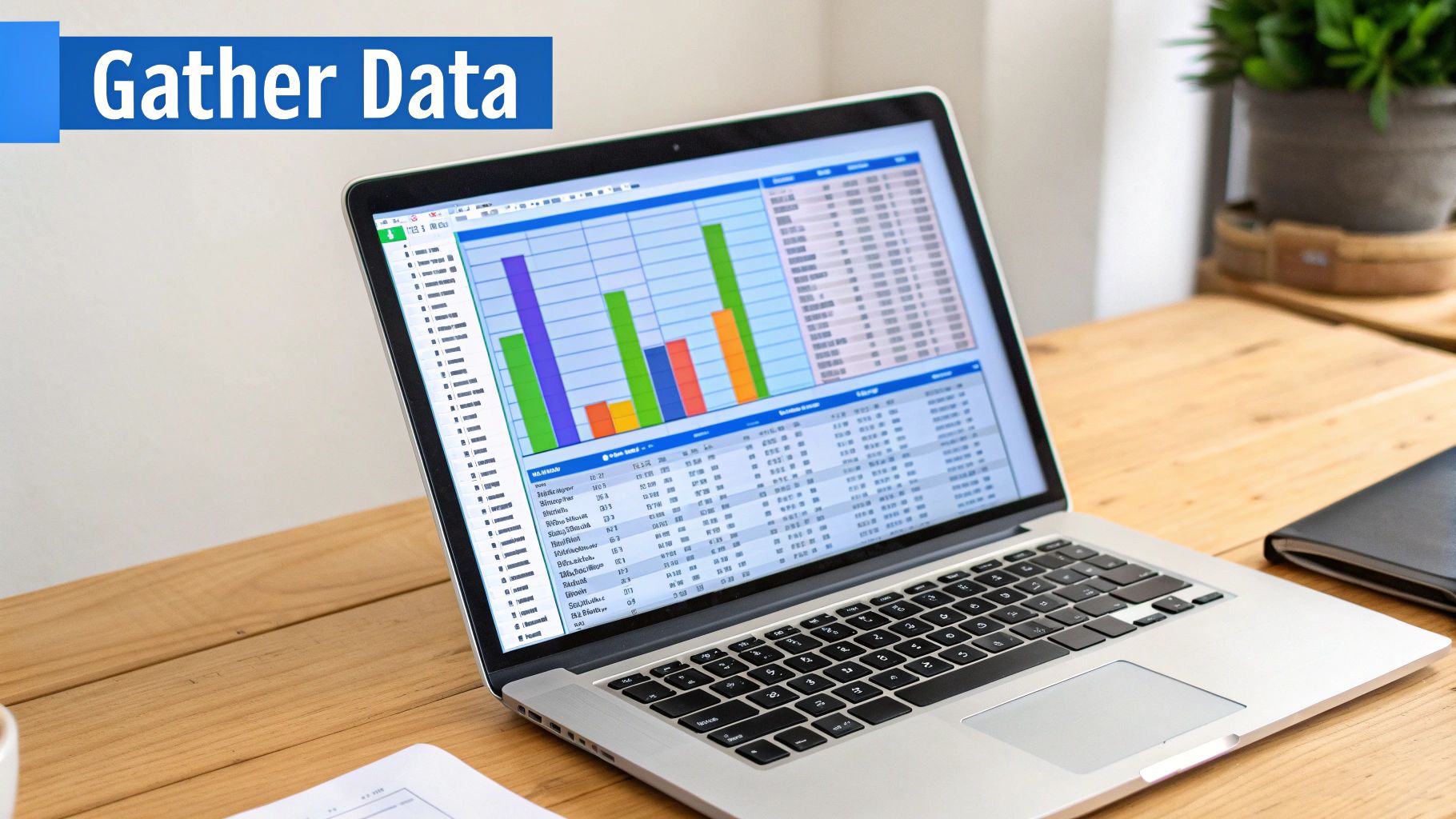
Setting Up Your Data
First things first, you need the data. You can easily pull historical daily closing prices from sources like Yahoo Finance or even directly from your brokerage platform. For this walkthrough, let's pretend we're analyzing the last 30 trading days of TSLA.
You don't need any fancy software. A simple spreadsheet tool like Google Sheets or Excel is perfect for this. Just set up two columns: one for the Date and one for the Closing Price.
With your data laid out cleanly like this, you're ready for the actual calculations.
Calculating Daily Returns
Now that your prices are organized, the next move is to calculate the daily percentage return for each day. You'll skip the very first day, of course, since there's no previous day to compare it to.
The formula is pretty straightforward:
(Today's Close - Yesterday's Close) / Yesterday's Close
Create a new column in your spreadsheet right next to the closing prices and apply this formula all the way down. This will give you a series of daily returns—the raw material for our volatility calculation. These numbers simply show you how much the price moved each day, whether it was up or down.
Pro Tip: When you're just starting out, try sticking to a consistent lookback period, like 20 or 30 days. This gives you a good feel for recent market action without getting thrown off by a single noisy day. As you get more comfortable, you can start experimenting with longer or shorter timeframes.
Finding the Standard Deviation
Next, we need to measure how spread out those daily returns are. For that, we use the standard deviation formula. In any spreadsheet program, you can just use the STDEV function and apply it to your entire column of daily returns.
The number it spits out is your daily historical volatility. A higher number means the price swings were wilder; a lower number suggests a period of relative calm.
Annualizing for Comparison
A daily volatility figure is helpful, but it's tough to use for comparisons. To make it truly useful, we need to annualize it.
The standard practice is to multiply your daily volatility by the square root of 252, which is the approximate number of trading days in a year.
- The Formula:
Annualized Volatility = Daily Volatility * SQRT(252)
The result is your annualized historical volatility, which is usually shown as a percentage. For example, an annualized volatility of 35% for TSLA means the market expects its price to fluctuate within a 35% range (up or down) over the next year. This standardized number is what allows you to compare risk between completely different stocks, indices, or even asset classes.
When you're first learning to calculate historical volatility, the simple percentage change method is a great place to start. It gets the job done. But if you want to level up your analysis and get a more mathematically sound picture, it’s time to switch to logarithmic returns, or log returns.
Professionals prefer this method for a reason. It's not just about using a fancier formula; it provides a much more accurate view, especially when you're analyzing longer timeframes or dealing with assets known for massive price swings.
Here's why the simple percentage method can sometimes be misleading. Imagine a stock drops 50%, falling from $100 down to $50. To get back to where it started, it needs to rally 100%. Simple returns treat these as moves of different magnitudes, which isn't quite right. Log returns, on the other hand, see them as equal but opposite moves, which better reflects the underlying volatility.
This approach essentially normalizes the data, making price changes comparable across different time periods and asset prices.
The Power of the Natural Log
To calculate log returns, we'll use a slightly different formula that involves the natural logarithm (ln). It might look a bit intimidating at first, but plugging it into a spreadsheet is just as easy as the simple return calculation.
Here's the formula you'll use for a single day:
Log Return = ln(Today's Price / Yesterday's Price)
The real beauty of this method is that log returns are additive over time. You can just sum up the daily log returns to get the total return over a week, a month, or a year. You can't do that accurately with simple percentages. This property makes them the gold standard for any serious financial modeling or backtesting work.
Using log returns is a subtle but powerful upgrade to your analysis. It helps ensure that your volatility calculation isn't skewed by the compounding effects of large price moves, giving you a more reliable and stable metric.
The standard industry approach incorporates these logarithmic returns to better capture this compounding effect. First, you calculate the daily log return using the ratio of consecutive closing prices. After you have a series of these daily returns, you find the sample standard deviation and then annualize it by multiplying by the square root of 252. You can find more details on how to calculate historical volatility this way and see why it’s the preferred method for pros.
Applying Log Returns to Our Dataset
Let's go back to our previous dataset and put this into practice. In your spreadsheet, you'll want to create a new column right next to your simple returns column.
Instead of the old formula, you'll use this one:
=LN(Today's Price / Yesterday's Price)
Once you've calculated the log return for each day in your dataset, the rest of the process is exactly the same as before.
- Calculate the Standard Deviation: Use the
STDEVfunction on your new column of daily log returns. This gives you the daily volatility. - Annualize the Result: Multiply that daily volatility figure by the square root of 252. That's your annualized volatility.
When you compare the results from the simple returns method and the log returns method, you'll probably see a slight difference. For most stocks over short periods, this difference will be minor.
However, for highly volatile assets like cryptocurrencies or for any analysis that spans several years, the log return method provides a much more robust and accurate measurement of risk. This is the figure that quantitative analysts and professional traders rely on every day.
Beyond the Basics: Advanced Volatility Estimators
Relying only on closing prices is like watching a movie but only seeing the final frame of each scene. Sure, you get the general idea, but you miss all the drama—the tension, the reversals, the real story that happened in between. This is where more advanced methods for calculating volatility come in, giving you a much richer, more accurate picture of an asset’s true risk profile.
These estimators move beyond the simple close-to-close model by incorporating more intraday data. By looking at what happens during the trading day, they capture the full extent of an asset's price swings, providing a more sensitive and often more useful measure of its behavior.
Capturing Intraday Action with the Parkinson Number
One of the most effective and well-regarded advanced estimators is the Parkinson volatility estimator. Instead of looking at closing prices, it focuses exclusively on the daily high and low. This shift in perspective is incredibly powerful.
Imagine a stock that opens at $100, soars to $105, plummets to $95, and then closes right back at $100. A standard close-to-close calculation would show a daily return of 0%, suggesting no volatility at all. Yet, that stock experienced a wild 10% price range during the day. The Parkinson method is designed specifically to capture this hidden action.
More advanced estimators can offer a significant edge. The Parkinson method, for instance, uses the difference between daily high and low prices, calculating volatility based on the squared logarithm of their ratio. Empirical analysis shows that this approach can be up to five times more efficient than standard measures because it doesn’t ignore the full price journey within a trading session. If you want to dive into the stats, you can find a deeper analysis of historical volatility measurement that backs this up.
This isn't just academic—it has direct, practical applications for traders looking for an edge.
From my own experience, using a high-low estimator like Parkinson is especially useful for assets prone to sharp intraday reversals. It acts as an early warning system, highlighting building pressure long before it might show up in the daily closing price.
Incorporating More Data with Garman-Klass
For those who want an even more complete picture, the next logical step is the Garman-Klass volatility estimator. This method takes things further by incorporating the open, high, low, and close (OHLC) prices into its formula. By using all four of these key data points, it aims to provide one of the most statistically efficient estimates of historical volatility possible.
These sophisticated models give you a few key advantages:
- Increased Efficiency: They extract more information from the exact same daily data.
- Greater Sensitivity: They react much more quickly to changes in intraday trading patterns.
- Improved Accuracy: They provide a more robust measure of an asset's true price dispersion.
These are the kinds of tools that quants and algorithmic traders use to refine their models. While they require slightly more complex math, understanding the principles behind them can dramatically improve your market analysis and lead to much more effective strategies. Mastering these methods is a key part of developing advanced volatility trading strategies for 2025.
Visualizing Volatility for Faster Trading Decisions
Doing the math is one thing, but making sense of it in the heat of a trading session is what really matters. Once you get the hang of calculating volatility, the next step is bringing that data to life on your charts. This is where you shift from being a mathematician to a market tactician, turning abstract numbers into real, actionable trading signals.
Forget about plugging numbers into a spreadsheet every day. Modern platforms like ChartsWatcher let you pop a Historical Volatility indicator onto any chart with a single click. It automates the entire process, freeing you up to focus on reading the market instead of running calculations.
From Numbers to Actionable Insights
With the indicator on your screen, you can start hunting for patterns that manual calculations could never reveal. The goal is to see exactly how changes in volatility influence price action in real-time.
For example, a classic pattern I always watch for is a sudden spike in volatility after a long, quiet period of consolidation. More often than not, this is a giant flare telling you a major price move is brewing. It’s like the market is coiling up for a big breakout, and the volatility indicator is your heads-up.
Here’s a look at the ChartsWatcher platform, which shows how you can pull together various tools, including visual indicators, to create a complete analytical dashboard.
This kind of integrated view lets you see volatility metrics right alongside price action and other critical data, which makes for much faster and sharper decision-making.
Reading the Volatility Story
Another critical insight comes from watching volatility die down. When you see the indicator trending lower, it often means an asset is entering a period of balance or consolidation. That could be your cue to tighten up stop-losses or get ready for a range-bound trading environment.
My personal rule is pretty simple: when volatility is high and expanding, I'm on the lookout for breakouts and trend-following opportunities. When it's low and contracting, I shift my focus to mean-reversion strategies or just stay on the sidelines and wait for a better setup.
By making this kind of visual analysis a core part of your routine, you’ll build a much more intuitive feel for the market’s rhythm.
Integrating Volatility into Your Workflow
Putting visual volatility analysis into practice is straightforward but incredibly powerful. Here are a few ways I like to integrate it into my daily trading toolkit:
- Confirm Breakouts: Use a sharp jump in volatility to confirm the strength of a price breakout from a key support or resistance level. A breakout with no volatility behind it is often a fake-out.
- Identify Complacency: Extremely low volatility can signal market complacency, which often comes right before a sharp, unexpected reversal. It’s the quiet before the storm.
- Time Your Entries: I often wait for volatility to start picking up before entering a trade. This helps improve the odds that I'm not jumping into a dead market and that I’ll catch a strong move.
Ultimately, plotting volatility directly on your chart transforms it from a lagging statistical number into a dynamic, forward-looking tool. It helps you anticipate where the market might be headed instead of just reacting to where it's been, giving you a critical edge.
Got Questions About Trading With Volatility?
Once you start crunching the numbers on volatility, you'll find that a bunch of practical questions pop up almost immediately. Working through these is what separates traders who just have data from those who have a real edge.
Let's walk through some of the most common things traders ask when they first start putting these powerful concepts to work. The answers aren't always cut and dry—they usually circle back to your own trading style and what you're trying to accomplish.
What's the Best Time Period for This Calculation?
There’s no magic number here. The "best" period is simply the one that lines up with how long you plan to be in a trade.
A short-term day trader, for instance, might be laser-focused on a 10 or 20-day historical volatility. This gives them a very sensitive read on the market's current mood, reacting quickly to news and price swings.
On the other hand, a swing trader or a long-term investor is going to want to zoom out. They'll probably look at 60, 90, or even 252 days of data. This longer window smooths out all the daily chatter and gives a clearer picture of the asset's typical, more stable volatility over time. The goal is to match your analytical lens to your trade's expected lifespan.
Why Is Volatility So Different Across Asset Classes?
You'll quickly notice that volatility varies wildly between stocks, forex, and crypto. This comes down to a few key things, like market size, how easily you can buy or sell (liquidity), and how much regulation is involved.
A massive, blue-chip stock like Coca-Cola is way less volatile than a small-cap biotech firm because its market is incredibly deep and mature. There are just too many buyers and sellers for the price to get thrown around easily.
The forex market, meanwhile, dances to the beat of macroeconomic news and what central banks are doing, which creates its own unique rhythm. And then there's crypto—a newer, more speculative world where extreme volatility is driven by fast-moving tech changes and wild swings in investor sentiment.
High volatility isn't something to fear. Think of it as a double-edged sword: it creates huge opportunities but also carries significant risk. The best traders don’t run from it; they respect it and build strategies that can handle it.
How Can I Use Volatility to Set My Stop Losses?
This is one of the most practical ways to use volatility, hands down. Instead of picking an arbitrary percentage for your stop-loss, you can tie it to a real-time volatility metric like the Average True Range (ATR). This makes your risk management dynamic and smart, adapting to what the market is actually doing right now.
For example, a common approach is to set your stop-loss at 2x the current ATR below your entry price. Here’s why that’s so effective:
- When volatility is high: Your stop will naturally be wider. This gives your trade more room to breathe and helps you avoid getting knocked out of a perfectly good position by random market noise.
- When volatility is low: Your stop will be much tighter. This helps you lock in profits and protect your capital more effectively as the market chops around in a narrow range.
Basing your stops on volatility is a cornerstone of any solid trading plan. To really dig into this, our definitive guide to risk management and trading covers these techniques in much more detail. After all, learning to manage risk properly is just as important as calculating volatility in the first place. This strategy keeps your risk parameters perfectly in sync with the market's behavior.
Ready to stop calculating and start analyzing? ChartsWatcher provides powerful, real-time volatility indicators and a fully customizable dashboard to give you a critical edge.